Procedure

Procedure for simulator

Controls

• Start button: Starts the experiment.
• Switch on: Turns on the laser.
• Select Fiber: Selects the type of fiber used.
• Select Laser: Selects a different laser source.
• Detector distance (Z): Use the slider to vary the distance between the source and the detector (i.e., toward or away from the fiber).
• Detector distance(x): Use the slider to change the detector position (i.e., move left or right with respect to the fiber).
• Show Graph: Displays the graph.
• Reset: Resets the experimental setup.

Preliminary Adjustment

Drag and drop each apparatus in to the optical table as shown in the figure below.

• Then Click “Start” button.
• Switch On (now you can see a spot in the middle of the detector)
• After that select the Fiber and Laser for performing the experiment from the control options.

To perform the experiment

• Set the detector distance Z (say 4mm). We referred the distance as “d” in our calculation.  
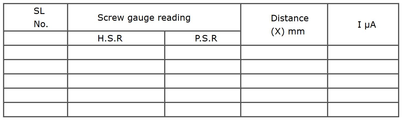
• Vary the detector distance X by an order of 0.5mm, using the screw gauge (use up and down arrow on the screw gauge to rotate it).
• Measure the detector reading from output unit and tabulate it.
• Plot the graph between X in x-axis and output reading in y-axis. See figure 5.
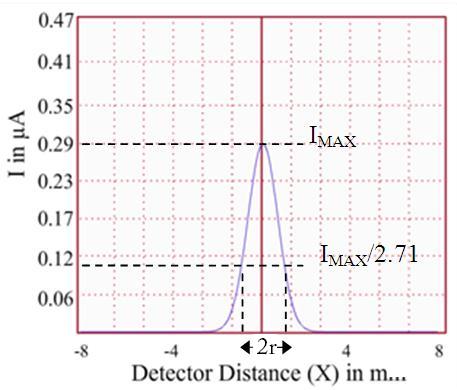
• Find the radius of the spot r, which is corresponding to Imax/2.71 (See the figure 5).

• Then find the numerical aperture of the optic fiber using the equation (4).

Observation column

Calculations

istance between the fiber and the detector, d = …………………………… m
Radius of the spot, r =……………………….. m
Numerical Aperture of the optic fiber, $sin(θ)=\frac{r}{\sqrt{r^{2}+d^{2}}}$ = .................
Acceptance angle, $θ={sin^{-1}}\left ( \frac{r}{\sqrt{r^2+d^2}} \right )$ = ...............

Result

Numerical aperture of the optic fiber is = …………………
Angle of acceptance = ……………….